In the last tutorial, we briefly mentioned some insights about the big O notation. Yet, in this tutorial, we’re going to simplify big O notation in data structure with examples in much more detail.
In 1976, Niklaus Wirth wrote a book and named it,
Algorithms + Data Structures = Programs
This gives us an understanding of to what extent data structures and algorithms are inseparably related.
After all, we — developers — are building programs that are a result of combining data structures and algorithms. And we are, obviously, meant to build efficient ones. Right?
But how can we tell if a program is effective at the level of lines of code and execution?
If you’re ready to follow up, I hope that you’ll get a satisfying answer to this question in the remaining lines of this writing…
Some Concepts…
In the previous tutorial, we listed some of the basic operations of data structures, but we never talked about the nature of these operations. What really are they?
The short answer, these operations fall under the umbrella of what we call “algorithms”…But…Hey…
# What’s an Algorithm?
An algorithm is a solution to a specific problem. It is actually a procedure that represents a finite set of instructions, written in order to accomplish a certain predefined task.
An algorithm is written in a natural language, which means that you can write it in any non-artificial way. But most likely, you’re going to use a Flowchart or a Pseudo-code to describe it.
When you use an artificial language — programming language — to translate algorithms into code(s), they become solutions that your machine can run.
But here’s the thing…We often hear them say, there’re multiple solutions to every problem. Actually, they’re right!
Now, you and your friend might write different algorithms for the same problem…Yet, another question might arise now…
# What’s a Good Algorithm?
How can we tell that your algorithm is better/worse than your friend’s one?
Remember, you’re going to translate your solution into lines of code with your preferred programming language and feed it to your machine hoping that it’s going to provide you with some output.
You got different machines. Yours is more powerful in terms of the time of execution and storage.
Let’s say that you guys have been told to write a solution that is going to tell your machines to turn on the light in a given bedroom a half-hour before 9 pm.
To try your solutions out, we want to turn on the lights in your bedroom (yours: one bedroom). After running the solutions on your machines, you both were on time, and both of you win. Congrats!
Now, we need you to turn on the light in all bedrooms in your city. Let’s do it…
After running the solutions for the bedrooms in the whole city. You were on time, but your friend’s solution went beyond 9 pm and couldn’t turn on all the lights…
Does that mean that your solution is better? is it a more scalable solution in terms of time and space? I’m sorry to tell you this, but not necessarily…Because we most likely want your solutions to be universal and can run effectively no matter what machine we’re using, no matter how many bedrooms in the world we want them to turn on lights in…Your friend’s solution might run better on a more powerful machine (maybe even on your machine)…
Now to end up this fight, we’ve got two solutions to measure the performance of your algorithms and tell which is better. So, whether
- We’re going to practically test your solutions on all machines around the globe and make a final assumption about which one is more performant. Can we do that? Never…It’s impossible.
- Or, we can find a theoretical way as a shortcut to describe the behaviour of your solutions. Hopefully, we have something called the big O notation that we can use to achieve that.
The big O notation…
Big O notation is a mathematical method we use to measure the complexity of an algorithm. Therefore, we can tell how well it scales in terms of the time or space required to solve the problem with a larger number of inputs.
The big O notation is denoted by the letter“O”. It represents the upper bound of an algorithm’s time/space complexity. The following chart illustrates the different cases in which an algorithm’s complexity might fall into.

[modified image] source of the original image here
We can see that the time/space complexity changes accordingly to the input size denoted by the letter “n”. The more the curve goes up the more the complexity increases.
You would always try to look up the complexity of O(n) and below if you want your solution to be called “fair”, “good” or “excellent”. A complexity of O(n * log n) and above is considered to be “bad” and might be “horrible”. Therefore, you should always try your best to avoid these — In some cases, you might find yourself obliged to be in the O(n * log n) and that’s okay. But, more than that, it’s to be in the red zone…
Time Complexity Calculation
When it comes to time complexity, we’re not going to use a timer to make calculations. However, we’re going to measure time relatively by counting the number of operations done in function of the input size.
Let’s see the following examples to learn how to calculate the time complexity of an algorithm.
But before we hit the examples, I’ve got something for you. Since the following examples are made in JavaScript, you might probably be interested in my online course to learn JavaScript from the ground up. It’s FREE and FOREVER!

Learn JavaScript from Scratch for FREE
This course will teach you modern core JavaScript from the basic fundamentals to advanced topics. It is intended to make you learn JavaScript from scratch apart from its use for frontend/backend development or whatever. It aims mainly to give you an opportunity to build a solid foundation to become a better JavaScript developer no matter# Example 01: The Constant Complexity O(1)
Let’s say that we want to say “Hi” to the first person on our list of people…
const people = ['A', 'B', 'C', 'D', 'E'];
console.log("Hi " + people[0]); // executes only once no matter how large is our list of people
In this example, no matter how many people we have in our array, it would always do the operation of greeting only once.
If we would like to represent that by a graph, it would look something like the following,

You can easily notice that the time complexity is “constant” in this case. And we usually denote it as “O(1)”.
# Example 02: The Linear Complexity O(n)
This time, we want to say “Hi” to everyone on the list…
const people = ['A', 'B', 'C', 'D', 'E'];
for(let i = 0; i < people.length; i++){
  console.log("Hi " + people[i]); // operation 1: repeats "people.lenght" times
}
So, in our example, we would repeat line 3 (operation 1) our array’s length times (5 times). Moreover, we would repeat it 10 times if we had an array of 10 elements, 1000 times for an array of 1000 elements, and so on…
Again, the representation by a graph would look like the following,

You can notice that the complexity increases linearly. The reason why this type of complexity is often called “Linear” and denoted as “O(n)”.
# Example 03: The Linear Complexity O(n²)
In this example, we want to display every possible pair in the array group.
const group = ['A', 'B', 'C'];

for (let i = 0; i < group.length; i++) {
  for (let j = 0; j < group.length; j++) {
    console.log("(" +group[i] + ", " + group[j] + ")"); // This operation would repeat 9 times which is (group1.length * group1.length = group1.length^2)
  }
}
Here, we’re using two nested loops to solve the problem. As a result, we would get line 6 repeated 9 times which is the result of the group.length square.
If we would like to represent the complexity of this solution with a graph, we would have this,

Scaling the array will always lead to repeating the operation at line 6, n*n times (Assuming that n is the length of the array). This gives us what we call a “quadratic” time complexity. And it is often denoted as “O(n²)”.
We usually get a quadratic time when we use nested loops. As we’ve mentioned above, you should do your best to avoid this kind of complexity.
# Example 04: The Logarithmic Complexity O(log n)
In the logarithmic complexity which is usually denoted by “O(log n)”, when the input size scales, the number of operations (relatively time) scales much slower.
An example of that would be the Binary Search algorithm — we‘ll cover this type of algorithm in much more detail in the upcoming tutorials.
# Example 05: The Logarithmic Linear Complexity O(n * log n)
The logarithmic linear complexity which is usually denoted by “O(n * log n)” comes in between the quadratic(worse) and the logarithmic one(better).
Examples of such type of complexity can be seen in the sorting algorithms generally.
# Example 06: The Exponential Complexity O(2^n)
In the exponential complexity, the execution time doubles every time as the input size grows.
An example of that would be solving the power problem “c(x,y)” using a recursive approach.
# Example 07: The Factorial Complexity O(n!)
We end up having a factorial complexity whenever we do calculations for permutations and combinations. Generally, we’re adding a loop for every element.
An example of that would be the complexity of The Traveling Salesman problem.
Space Complexity Calculation
The space complexity of an algorithm can fall in the same cases as the time complexity. However, when it comes to its calculation, we take into consideration the memory allocated by the algorithm instead of the number of operations done.
When we say memory allocated by the algorithm, we mean two types of memory allocation,
- Space used by the algorithm input(s)
- The auxiliary space. It refers to the temporary space used by the algorithm to solve the problem. Examples of that would be using temporary variables and function calls.
Let’s have an example for illustration,
In this example, we want to say “Hi” 10 times…
var n = 10; // O(1) for n
for (let i = 0; i < n; i++) { //O(1) for i {temporary variable}
  console.log('Hi');
}

// O(1 + 1) = O(2) => can be simplified to O(1)
As you can see, we have a variable n which is going to have a constant space complexity of O(1) since we’re going to allocate it once no matter how large our input n is. The same applies to variable i which is an auxiliary variable. So, we’ll end up with a space complexity of O(1+1) = O(2). The space of this algorithm stays constant no matter how large is our input size. Therefore, O(2) can simply be simplified to O(1) — We’ll look at how to simplify calculations in the next section.
Big O Calculation Rules
There are some rules you should consider when calculating Big O. These can be summed up in the following points,
1) Big O is always calculated for the worst-case scenario.
2) Add up the Big O of each operation together with different terms for different inputs.
3) Remove constants
4) The dominant term is the Big O of the algorithm. Drop the rest…
If it doesn’t make sense, no worries. Here’s an example,
const arr1 = [1, 55, 58, 3, 2]; // O(1)
const arr2 = ['a', 'b', 'c', 'd', 'e']; // O(1)
let x = '58'; // O(1)

//find  x in arr2 and print its index => O(n)
for (let i = 0; i < arr1.length; i++) {
  if (arr1[i] == x) {
    console.log(i);
    break;
  }
}

//print all possible pairs in arr2 => O(p^2)
for (let j = 0; j < arr2.length; j++) {
  for (let k = 0; k < arr2.length; k++) {
    console.log(arr2[j], arr2[k]);
  }
}
The example itself doesn’t make sense, I know. But, here’s we’re just trying to check on the use of the Big O rules…
- Rule 01: we’re considering the worst-case scenario. Look at the first loop, in our case, the element is found at the half of the array. However, because we’re calculating Big O, we assume that the worst-case is that x is found at the last index of the array.
- Rule 02: we’re going to add up the Big O of each operation together with different terms for different inputs. In fact, in our example, we got two loops applied on two different inputs (arr1 and arr2). So, we define n for arr1 and p for arr2 to denote the Big O. The result of our calculation at this step would be something like the following,
O(1+1+1+n+p²) = O(3+n+p²)
- Rule 03: let’s remove any constants. The result this time would be,
O(3+n+p²) => O(n+p²)
- Rule 04: finally, let’s keep only the highest-order term and drop the rest. So, p² is the dominant part of the equation. We end up having something like the following as the final Big O of our nonsense algorithm,
O(n+p²) => O(p²) => O(n²) — A quadratic time complexity
Big O Cheatsheet
To finish up this post, I want to share with you the following cheat-sheet that you might refer to from time to time to decide about the right data structure to use to solve a particular problem.

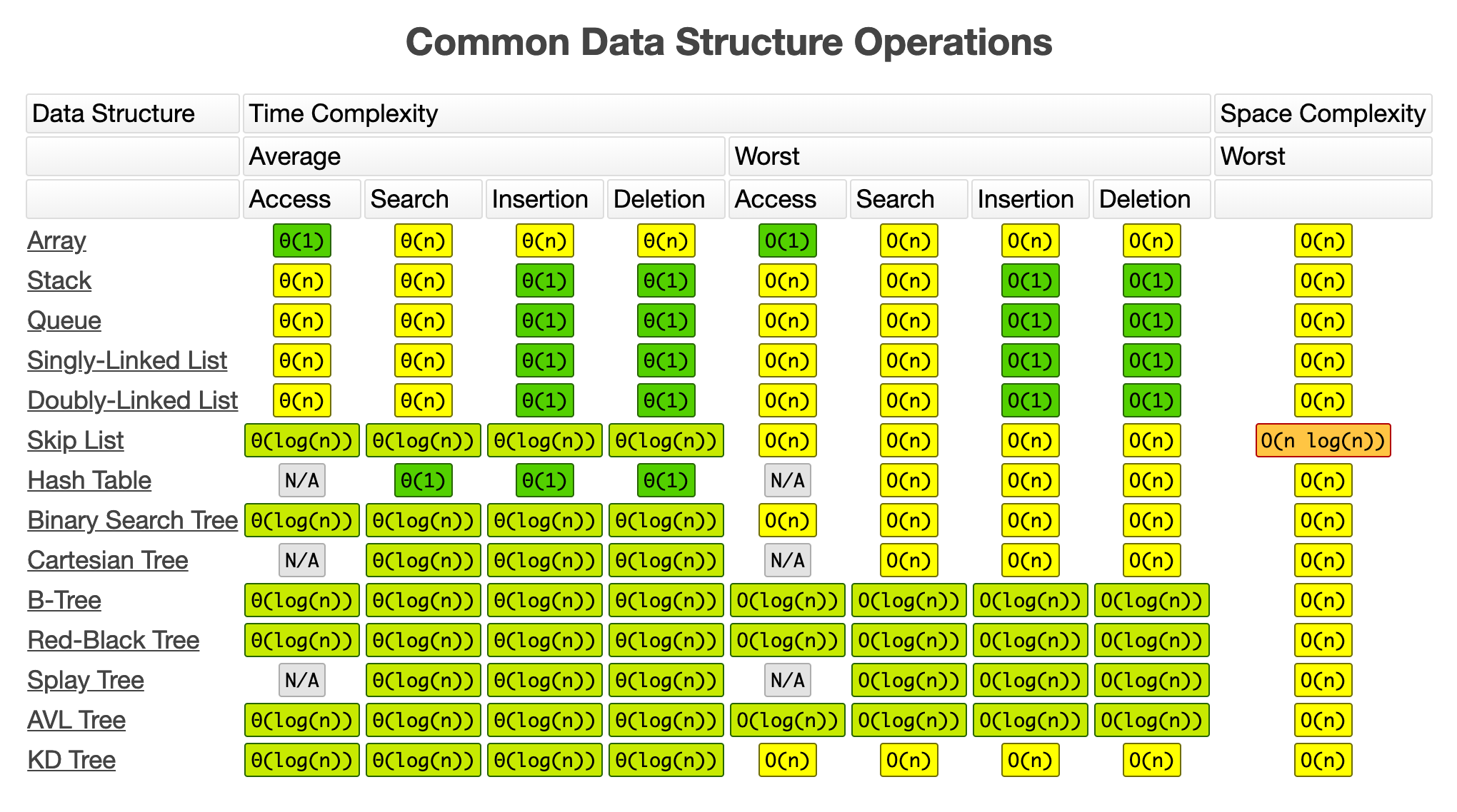
Basically, this is it for the basics of Big O notation.
in this blog post, we have covered the essential parts of what you usually need. Nevertheless, you might find an in-depth explanation of it in other resources if you’re still curious.
If you have any questions or feedback, please, use the comment section. And stay tuned for upcoming tutorials…
Wait for a second, please! Before we leave, if you want, let’s connect…